Multivariate anomaly detection

This tutorial shows you how to train a multivariate anomaly detection model in a Fabric notebook by using sample data stored in an eventhouse. You then use the trained model in a KQL queryset to score new data and visualize anomalies.

For background information, see Multivariate anomaly detection in Microsoft Fabric - overview.

Prerequisites

A workspace with a Microsoft Fabric-enabled capacity.
An Admin, Contributor, or Member workspace role. You need this permission level to create items such as an environment.
An eventhouse in your workspace with a database.
The sample data file.
The sample notebook.

Part 1: Turn on OneLake availability

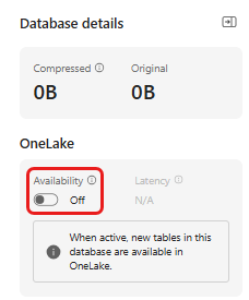
Turn on OneLake availability before you load data into the eventhouse. This setting makes the ingested data available in OneLake so that you can access the same table from a notebook later in the tutorial.

In your workspace, open the eventhouse that you created in the prerequisites, and then select the database where you want to store your data.
In the Database details pane, set OneLake availability to On.

Part 2: Turn on the KQL Python plugin

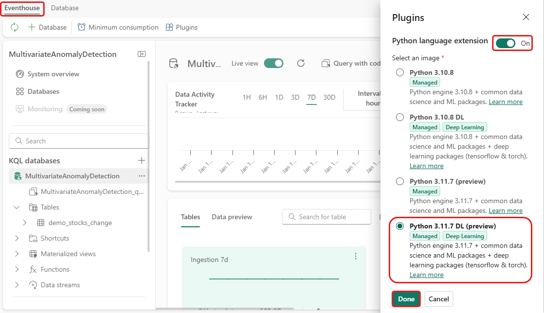
In this step, you turn on the Python plugin in your eventhouse. This step is required to run the Python code in the KQL queryset in Part 9: Predict anomalies in a KQL queryset. Select the Python image that includes the time-series-anomaly-detector package.

In the eventhouse, select Eventhouse > Plugins on the ribbon.
In the Plugins pane, set Python language extension to On.
Select Python 3.11.7 DL.
Select Done.

Part 3: Create a Spark environment

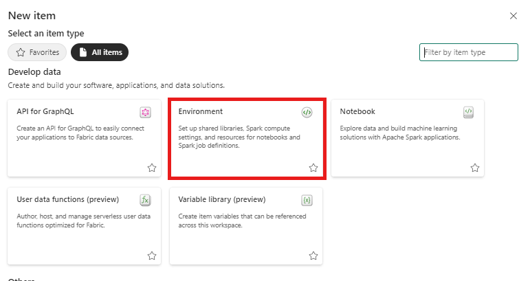
In this step, you create a Spark environment to run the notebook that trains the multivariate anomaly detection model. For more information, see Create and manage environments.

From your workspace, select + New item, and then select Environment.
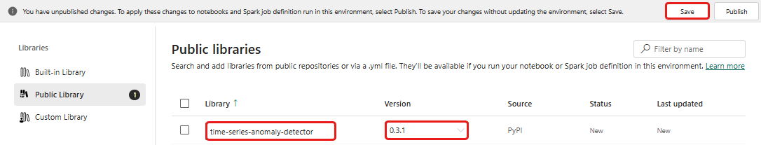
Enter MVAD_ENV for the environment name, and then select Create.
Under Libraries, select Public libraries.
Select Add from PyPI.
In the search box, enter time-series-anomaly-detector. In the Version box, enter 0.3.9.
Select Save.
Select the Home tab in the environment.
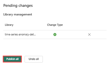
Select the Publish icon from the ribbon.
Select Publish all. This step can take several minutes to complete.

Part 4: Load data into the eventhouse

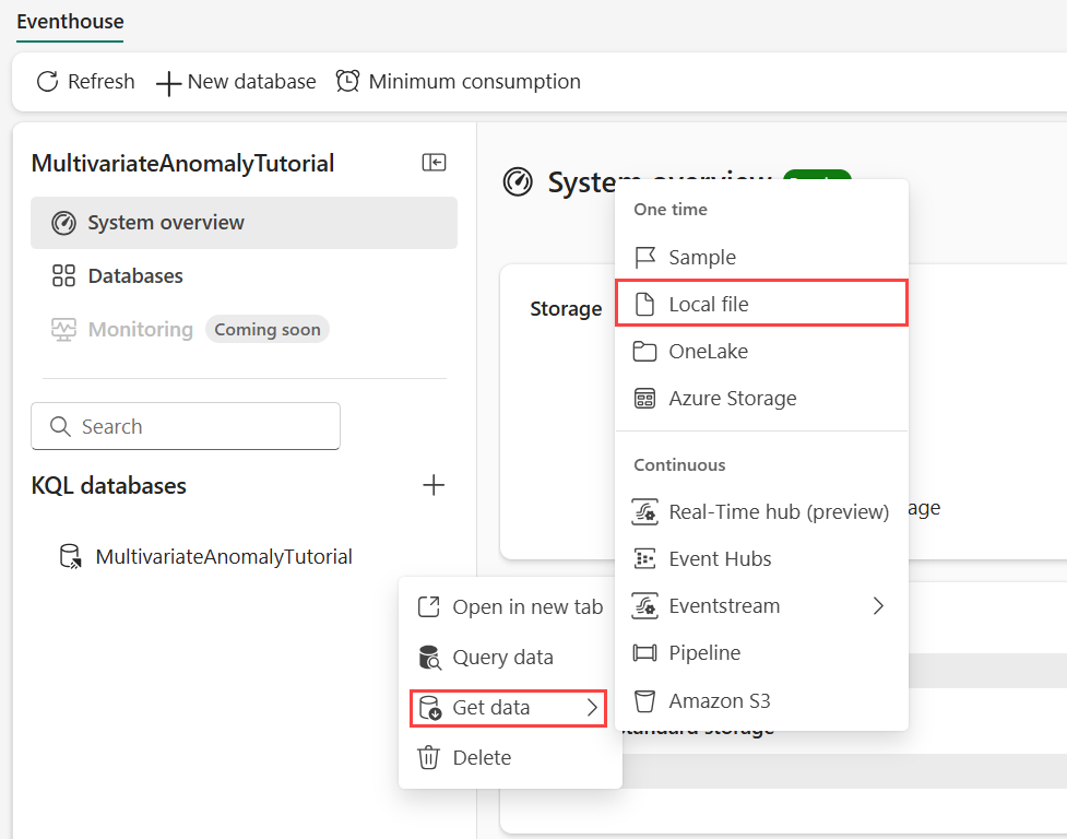
In the eventhouse, hover over the KQL database where you want to store your data, and then select More menu [...] > Get data > Local file.
Select + New table, and enter demo_stocks_change as the table name.
In the upload dialog, select Browse for files, and upload the sample data file that you downloaded in Prerequisites.
Select Next.
In the Inspect the data section, verify that First row is column header is set to On.
Select Finish.
When the data is uploaded, select Close.

Part 5: Copy the OneLake path

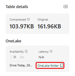
Select the demo_stocks_change table. In the Table details pane, select OneLake folder to copy the OneLake path to your clipboard. Save the path in a text editor for later use.

Screenshot of copying the OneLake path.

Part 6: Prepare the notebook

Select your workspace.
Select Import > Notebook > From this computer.
Select Upload, and choose the notebook you downloaded in Prerequisites.
After the notebook is uploaded, you can find and open your notebook from your workspace.
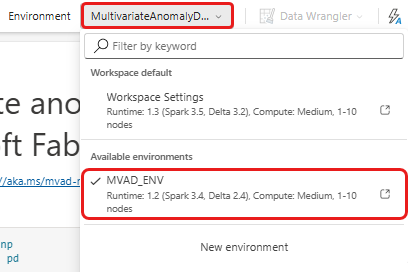
On the top ribbon, select the Workspace default drop-down list, and then select the environment you created in the previous step.

Part 7: Run the notebook

Import standard packages.
```
import numpy as np
import pandas as pd
```

Spark needs an ABFSS URI to securely connect to OneLake storage, so define a helper function that converts the OneLake URI to an ABFSS URI.

def convert_onelake_to_abfss(onelake_uri):
    if not onelake_uri.startswith('https://'):
        raise ValueError("Invalid OneLake URI. It should start with 'https://'.")
    uri_without_scheme = onelake_uri[8:]
    parts = uri_without_scheme.split('/')
    if len(parts) < 3:
        raise ValueError("Invalid OneLake URI format.")
    container_name = parts[1]
    path = '/'.join(parts[2:])
    abfss_uri = f"abfss://{container_name}@{parts[0]}/{path}"
    return abfss_uri

Replace OneLakeTableURI with the OneLake URI that you copied in Part 5: Copy the OneLake path, and then load the demo_stocks_change table into a pandas dataframe.

onelake_uri = "OneLakeTableURI"  # Replace with your OneLake table URI.
abfss_uri = convert_onelake_to_abfss(onelake_uri)
print(abfss_uri)

df = spark.read.format('delta').load(abfss_uri)
df = df.toPandas()
df['Date'] = pd.to_datetime(df['Date'])
df = df.set_index('Date').sort_index()
print(df.shape)
df.head(3)

Run the following cells to prepare the training and prediction dataframes.

Note

The actual predictions run in the eventhouse in Part 9: Predict anomalies in a KQL queryset. In a production scenario, you typically score new streaming data. In this tutorial, the dataset is split by date into training and prediction ranges to simulate historical and incoming data.
```
features_cols = ['AAPL', 'AMZN', 'GOOG', 'MSFT', 'SPY']
cutoff_date = pd.Timestamp('2023-01-01')
```
```
train_df = df.loc[df.index < cutoff_date, features_cols]
print(train_df.shape)
train_df.head(3)
```
```
train_len = len(train_df)
predict_len = len(df) - train_len
print(f'Total samples: {len(df)}. Split to {train_len} for training, {predict_len} for testing')
```

Run the cells to train the model and save it in the Fabric MLflow model registry.

from anomaly_detector import MultivariateAnomalyDetector
model = MultivariateAnomalyDetector()

sliding_window = 200
params = {"sliding_window": sliding_window}

model.fit(train_df, params=params)

model_name = "mvad_5_stocks_model"

import mlflow

with mlflow.start_run():
    mlflow.log_params(params)
    mlflow.set_tag("Training Info", "MVAD on 5 Stocks Dataset")

    model_info = mlflow.pyfunc.log_model(
        python_model=model,
        artifact_path="mvad_artifacts",
        registered_model_name=model_name,
    )

Run the following cell to get the registered model path that you use later for prediction in the KQL Python sandbox.

from mlflow.tracking import MlflowClient

client = MlflowClient()
mvs = client.search_model_versions(f"name='{model_name}'")
latest = max(mvs, key=lambda v: v.creation_timestamp)
model_abfss = latest.source
print(model_abfss)

Copy the model URI from the output of the last cell. You use it in Part 9.

Part 8: Create a KQL queryset

For general information, see Create a KQL queryset.

In your workspace, select + New item > KQL Queryset.
Enter MultivariateAnomalyDetectionTutorial, and then select Create.
In the OneLake catalog window, select the KQL database where you stored the data.
Select Connect.

Part 9: Predict anomalies in a KQL queryset

Run the following .create-or-alter function query to define the predict_fabric_mvad_fl() stored function:

.create-or-alter function with (folder = "Packages\\ML", docstring = "Predict MVAD model in Microsoft Fabric")
predict_fabric_mvad_fl(samples:(*), features_cols:dynamic, artifacts_uri:string, trim_result:bool=false)
{
    let s = artifacts_uri;
    let artifacts = bag_pack('MLmodel', strcat(s, '/MLmodel;impersonate'), 'conda.yaml', strcat(s, '/conda.yaml;impersonate'),
                             'requirements.txt', strcat(s, '/requirements.txt;impersonate'), 'python_env.yaml', strcat(s, '/python_env.yaml;impersonate'),
                             'python_model.pkl', strcat(s, '/python_model.pkl;impersonate'));
    let kwargs = bag_pack('features_cols', features_cols, 'trim_result', trim_result);
    let code = ```if 1:
        import os
        import shutil
        import mlflow
        work_dir = os.environ.get("UPLOAD_PATH")
        model_dir = work_dir + '/mvad_model'
        model_data_dir = model_dir + '/data'
        os.mkdir(model_dir)
        shutil.move(work_dir + '/MLmodel', model_dir)
        shutil.move(work_dir + '/conda.yaml', model_dir)
        shutil.move(work_dir + '/requirements.txt', model_dir)
        shutil.move(work_dir + '/python_env.yaml', model_dir)
        shutil.move(work_dir + '/python_model.pkl', model_dir)
        features_cols = kargs["features_cols"]
        trim_result = kargs["trim_result"]
        test_data = df[features_cols]
        model = mlflow.pyfunc.load_model(model_dir)
        predictions = model.predict(test_data)
        predict_result = pd.DataFrame(predictions)
        samples_offset = len(df) - len(predict_result)        # this model doesn't output predictions for the first sliding_window-1 samples
        if trim_result:                                       # trim the prefix samples
            result = df[samples_offset:]
            result.iloc[:,-4:] = predict_result.iloc[:, 1:]   # no need to copy 1st column which is the timestamp index
        else:
            result = df                                       # output all samples
            result.iloc[samples_offset:,-4:] = predict_result.iloc[:, 1:]
        ```;
    samples
    | evaluate python(typeof(*), code, kwargs, external_artifacts=artifacts)
}

Run the following prediction query. Replace enter your model URI here with the URI that you copied at the end of Part 7: Run the notebook.

The query detects multivariate anomalies across the five stocks by using the trained model, and then renders the results as an anomalychart. The anomalous points are displayed on the first stock (AAPL), but they represent anomalies in the joint behavior of all five stocks on a given date.

let cutoff_date=datetime(2023-01-01);
let num_predictions=toscalar(demo_stocks_change | where Date >= cutoff_date | count);   //  number of latest points to predict
let sliding_window=200;                                                                 //  should match the window that was set for model training
let prefix_score_len = sliding_window/2+min_of(sliding_window/2, 200)-1;
let num_samples = prefix_score_len + num_predictions;
demo_stocks_change
| top num_samples by Date desc
| order by Date asc
| extend is_anomaly=bool(false), score=real(null), severity=real(null), interpretation=dynamic(null)
| invoke predict_fabric_mvad_fl(pack_array('AAPL', 'AMZN', 'GOOG', 'MSFT', 'SPY'),
            // NOTE: Update artifacts_uri to model path
            artifacts_uri='enter your model URI here',
            trim_result=true)
| summarize Date=make_list(Date), AAPL=make_list(AAPL), AMZN=make_list(AMZN), GOOG=make_list(GOOG), MSFT=make_list(MSFT), SPY=make_list(SPY), anomaly=make_list(toint(is_anomaly))
| render anomalychart with(anomalycolumns=anomaly, title='Stock price changes in % with anomalies')

The resulting anomaly chart resembles the following image:

Clean up resources

When you finish the tutorial, delete the resources that you created to avoid unnecessary costs:

Browse to your workspace homepage.
Delete the environment created in this tutorial.
Delete the notebook created in this tutorial.
Delete the eventhouse or database used in this tutorial.
Delete the KQL queryset created in this tutorial.

Feedback

Was this page helpful?

Last updated on 2026-06-17